MoPSeq-DB allows users to i) navigate through all the genomic data related to mollusc pathogens, ii) access fully interactive views of genome structures, variants, and phylogenetic trees, and iii) download data in various formats : FASTA, GFF (General Feature Format), VCF (Variant Call Format), Newick phylogenetic tree, PNG.

The user-friendly platform provides a comprehensive overview of genomes and pathogens referenced in the database. Marine bivalve molluscs are infected by various pathogens, MoPSeq-DB visualisation tools are designed to fit each of their genome particularities. Thereby, MoPSeq-DB is suited to be used with viruses, bacteria and eukaryotes genomes.

In this page, MoPSeq-DB design is explain to facilitate exploration to the plateform users.

The sharing aspect of the project is based on the referencement of genomic data related to mollusc pathogens. It functions as a downstream repository for this data collected from public repositories for sharing genomes.



MoPSeq-DB shares four different files related to each referenced pathogen :

A FASTA, GFF, or VCF file can correspond to three different states of the genome assembly they are referring to :

• Complete - The complete genome of the sample.
• Non-redundant - A less complex complete genome, with only one copy of repeated regions (Delmotte-Pelletier et al. Virus Evolution, 2022.). The regions can also be re-organised depending on the pathogen.
• Partial - When the genome is only a fraction of the referenced genome/contig.

Thus, some samples may have several FASTA, GFF or VCF files.

For users, data sharing takes place within the Sequence Databases tab, in the navigation bar. When hovering over it, you can select the desired pathogen and see a table with the referenced data.

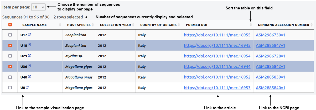
The main element of the page will be the table referencing the data. In this table, you have several direct functionalities, such as sorting the table based on the attribute of your choice or controlling the number of displayed lines.

The table's direct functionalities include:

The plateform offers dynamic data searching and filtering functionnaly, to be found above the table, in the following toolbar :

• Display - Enables you to select the list of attributes (metadata) that you want to display on the table.
• Filter - Provides different filtering possibilities, based on metadata, to apply to the table. You can combine multiple filters together.
• Download - Allows you to download the different files stored in the database. If a sample has multiple files of the same type, they will all be downloaded and differentiated with the tags "NR" for Non-redundant and "P" for Partial.
  The downloaded archive will also include a text file called not_found.txt if any of the requested files are not available.
• Search bar - You can use the search bar to match the information you entered with any referenced information. For example, entering "China" will display data referenced from China, while "Crassostrea gigas" will show all data with this host referenced.

The metadata fields used in MoPSeq-DB were designed to be as relevant and complete as possible in relation to pathogen analyses and attributes commonly found in databases like NCBI/EBI. MoPSeq-DB gathers up to 51 metadata fields corresponding to sample data, epidemiologic data, sequencing and assembling technical data, etc. You can download the MoPSeq-DB metadata template here.

Regarding missing values, they can be categorised as follows:

• Unknown - Information is missing.
• TBD - To Be Determined, the information will be filled at a later date.
• NA - Not Applicable, the information field is irrelevant to this particular sample.

On the platform, the 30 following metadata can be display and be used to filter genomes:

The update of MoPSeq-DB pathogen data is performed by regular crawling through the NCBI/EBI databases to retrieve new genomes of pathogen referenced in MoPSeq-DB. The plateform will also be regularly enriched with new pathogens as sequencing of mollusc pathogens progresses.
You can resquest for the addition of missing data by filling the form available in the Updates tab.
Currently under construction, there will also be the possibility for anyone to submit their own data if submission to GenBank/EBI is not planned. The submitted data will be first checked to ensure that the user metadata corresponds to the fields template of MoPSeq-DB before being reviewed by the maintenance team of the platform.

Data visualisation plays a significant role in interpreting genomic data. MoPSeq-DB adds value to other public sequence repositories by enabling data visualisation through interactive graphics. A set of scripts generate pre-proceded files allowing a dynamic visualisation of genomic information.
The visualisation aspect of the project can be divided into two sub-aspects : the visualisation of each sample's genomic information, and the creation of a phylogenetic tree from all genomes of a same pathogen.
-> Regarding the sample's genomic information, it can be visualised on the individual pages of each sample. To access these pages, users need to click on the value in the Sample Name attribute column in the data table (more information on the data table can be found here).
-> For the pathogen's phylogenetic placement, the visualisation will occur within the Phylogenies tab, in the navigation bar.

MoPSeq-DB visialisation tools are adapted to manage genomic data from various pathogens beyond mollusc diseases. Therefore, different type of graphs are generated to respond to the constraints corresponding to pathogens' different kingdoms.

The visualisation of the genomic structure is presented using an interactive graph that represents the different features recorded in the GFF file of the sequence. The various types of features are differentiated using a color code and positioned on different y-axis values to prevent overlap.
Each pathogen may have its own color code and representation characteristics based on what we consider most interesting to represent. For example, the structural regions of Ostreid herpesvirus-1 have different color representations, while the repeated regions have the same representation (see example below). New models of caracteristic representation can easily be defined as new pathogens are add to the platform.

The interactive graph displays labels such as the ORF number or region name when hovering over the represented elements. Additionally, the graph offers several options to the user, such as zooming on the x-axis (nucleotide positions), moving within the graph, selecting an element, and more.

Example of the graph and its functionalities:

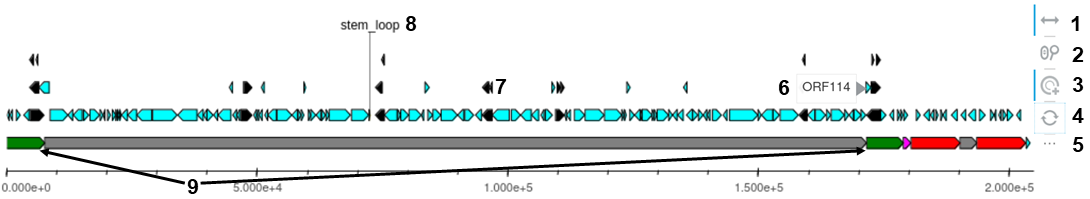
• Allow pan movement on the x-axis (active).
• Allow wheel zoom on the x-axis (non-active).
• Allow user selection of element (active).
• Refresh figure.
• Activate labels when hovering (active).
• Exemple of hovering label (here the name of a structural region).
• Exemple of GFF elements (CDS, genes, variations...).
• Due to its importance, the stem-loop region has a fixed label when present in the GFF file.
• Exemple of specific representation, here the two repaeated regions TRL and IRL have the same green color.

In MoPSeq-DB, most Vibrio aestuarianus chromosomes have been artificially created using RagTag to facilitate viewing, as bacterian genomes are more fragmented. Contigs obtained from the assembly have been regrouped, ordered, and oriented to form chromosomes based on complete reference genomes.

Three reference genomes have been utilised for this purpose:

• U17 for Vibrio aesturianus subspecies cardii
• 10_092_7MT1 for Vibrio aesturianus subspecies francensis
• 03008T for Vibrio aesturianus

Additionnal information has been calculated using GC_analysis and SkewIT. These analyses provide insights into the GC content and skewness of the genome, which can be valuable for understanding the characteristics and dynamics of Vibrio aestuarianus. 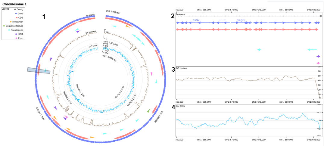Data is visualised on two scales:

• An overview of the chromosome linked to
• an interactive detailed one allowing to move horizontally on the graph, zoom on and get information of a selected element.
Complementary information is displayed:
• GC content
• GC skew along the genome.

Under development Based on the different VCF files, the frequency of detected variants and their coverage is represented using two interactive graphs. Similar to the genomic structure visualisation (see above), these graphs provide various options to the users. Additionally, there are buttons under the graph that allow users to hide the variation or reference labels.
Hovering over a label on the graphs will display either the position and frequency of the variation or the position and coverage depth, depending on the graph.

For most pathogens, it is possible to observe both inter-individual and intra-individual variations. Inter-individual variations represent the differences between the sample genome and the reference genome, while intra-individual variations represent the variations detected within the pool of reads used to assemble the sample's consensus sequence.

In the provided example graph, variation labels may overlap and be difficult to distinguish due to their close proximity in the sequence. However, users can easily isolate them by using available tools such as zooming and pan movement.

Example of the graph and its functionalities:

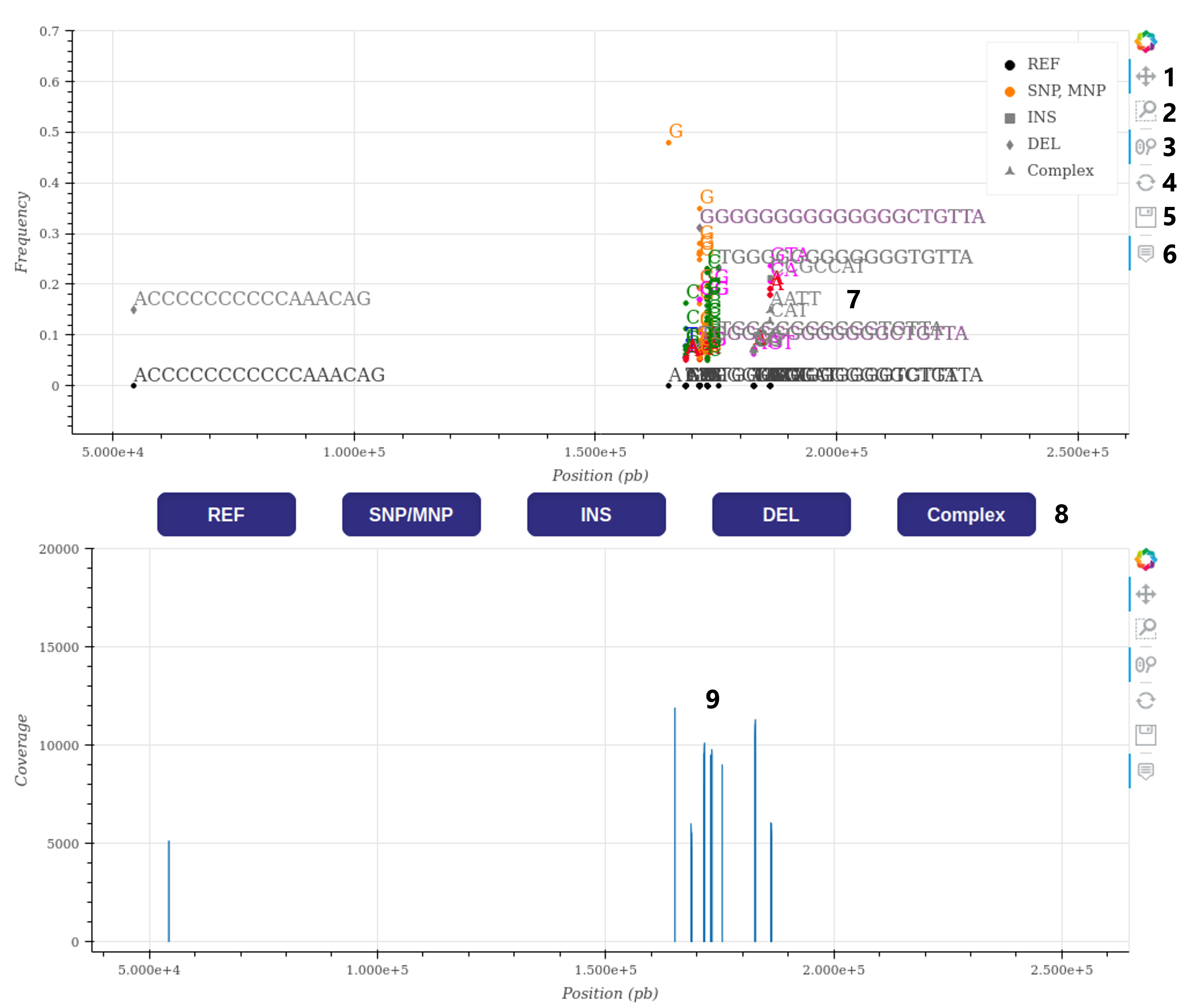
• Allow multi-directionnal pan movement (active).
• Allow box zooming (non-active).
• Allow wheel zoom on the x-axis (active).
• Refresh figure.
• Save a picture of the current graph.
• Activate labels when hovering (active).
• Exemples of variation labels : SNP are colored based on nucleotid, INDEL and complex are grey but differentiated by their labels form (see legend).
• Buttons to activate displaying of a type of label (all active).
• Exemple of variation coverage representation, coverage of inter-variations regions can also be displayed if the information is available in the VCF.

A phylogenetic tree is generated for each pathogen implemented in the plateform. The Phylogenies tab in the navigation bar redirects to an index page where the user can choose to see an interactive graph of the phylogenetic tree of all pathogen genomes of the database.
On the pathogen's phylogenetic tree page, which can be accessed through the Phylogenies tab or the link present on the sequence data page or sample information page, you will find a tree built with all available genomes of the pathogen.

Several ineractivity options are available on the toolbar above the table:

• Export - Allows you to download an image of the current tree with the selected or filtered nodes or edges in SVG format, or the tree file itself in NEWICK format.
• Informations - Displays an information box regarding the tree generation and model selection. This option assure the auditability of the calculation of the tree, information displayed are automaticaly saved in a report during tree generation.
• Selection - Provides a wide range of selection options for the tree, such as selecting leaf nodes or internal nodes.
• Search bar - You can use the search bar to search for specific sequences recorded in the tree.

Right below the toolbar, additionnal options are available:

To go futher, MoPSeq-DB amis to offer the possibility to increase the accessibility and the reproductability of genomic data analyses. Therefore, two additionnal functionnalities are planned to be include in the plateform. Under construction, this aspect operates with a pipeline based on the Evolutionary Placement Algorithm (EPA) of the RAxML software. Users can submit sequences, and the algorithm will suggest high-likelihood branch placements for them on the existing pathogen tree. The EPA algorithm allows for fast computing by applying maximum likelihood without reconsidering the entire phylogenetic tree. Under construction, this aspect is intended to integrate open-source modules from Nextstrain (Hadfield et al. Bioinformatics, 2018.) to enable near real-time epidemiology monitoring and phylogenetic visualisation of compatible pathogens registered in the database. This will allow the joint analysis of epidemiologic and genomic data, and thus extend the scope of the platform. Icons used in MoPSeq-DB are from icones8 website. Source code, documentation and docker container are available in the MoPSeq-DB GitLab repository. MoPSeq-DB dataset is available for direct access and loading through Sextant Catalog, a CoreTrustSeal certified data providing service from Ifremer : doi.org/10.12770/52134702-4bbd-4c63-af34-9a2cde28e0cc.

Go back to the top